Statistics with Python – Variance and Standard Deviation

In our previous lesson of the Geekswipe Statistics micro-course series, we learned about the measure of central tendency. We explored the concepts of mean, median, and mode.

In this lesson, we will explore the measure of dispersion, and the statistical methods used to measure it.

Measure of dispersion

While the measure of central tendency is focused towards the central aspects of the given dataset, the measure of dispersion is focused towards the span of the entire dataset. It measures or summarizes how spread the data is. The common measures of dispersion we are going to explore are variance and standard deviation.

Variance

We’ve seen that mean, median, and mode are used to find the central tendency of the data distribution. In other words, they help us to summarize the central values of the data. But centres can be the same for different datasets too. For example, consider these two lists.

[-300, -200, -100, -100, 0, 100, 100, 200, 300]

[-3, -2, -1, -1, 0, 1, 1, 2, 3]

Now if you were to find the mean and median for both the lists, it will be the same. Zero! Let’s do that quickly with Python.

import numpy as np
import pandas as pd
import matplotlib.pyplot as plt


# Data
sierra_points = np.array([-300, -200, -100, -100, 0, 100, 100, 200, 300])
tango_points = np.array([-3, -2, -1, -1, 0, 1, 1, 2, 3])

# Mean
print("Mean of sierra is: {}.".format(np.mean(sierra_points)))
print("Mean of tango is: {}.".format(np.mean(tango_points)))

# Median
print("Median of sierra is: {}.".format(np.median(sierra_points)))
print("Median of tango is: {}.".format(np.median(tango_points)))

# Plot
plt.subplot(121)
plt.title("Sierra")
plt.xlabel("Points")
plt.ylabel("Counts")
plt.xlim(-300, 700)
plt.ylim(0, 5)
plt.hist(sierra_points)
plt.axvline(np.mean(sierra_points), color='g', linestyle='dashed', linewidth=1)

plt.subplot(122)
plt.title("Tango")
plt.xlabel("Points")
plt.ylabel("Counts")
plt.xlim(-50, 50)
plt.ylim(0, 5)
plt.hist(tango_points)
plt.axvline(np.mean(tango_points), color='g', linestyle='dashed', linewidth=1)

plt.show()

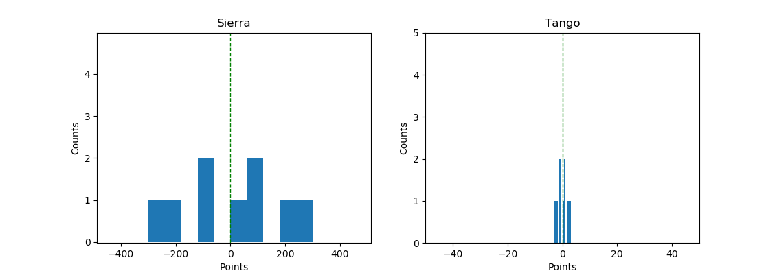
So, in this case, the measure of central tendency is worthless when you have to compare two different datasets. But look at how different the ‘spread’ is for these two data between -300 to 300. The first list is pretty stretched all the way from -300 to 300. The second list is tightly packed around -3 to 3. This measure of ‘how far the data is spread out or scattered across’ is called variance.

If we calculate the distance between the mean and each of the data points, we could get an idea of how scattered these data points are. Once we get the differences, the variance of the whole dataset is just the average of all the differences (squared to prevent negative numbers).

Mathematically, variance σ² can be expressed as follows.

\( \sigma^{2}=\frac{\sum_{i=1}^{N}\left(X_{i}-\mu\right)^{2}}{N} \)

Where X-μ is the difference between the data point X and mean μ, and N is the total number of differences.

Example

But thanks to Numpy, we can sit back, relax, and calculate the variance in a jiffy.

import numpy as np

# Data
sierra_points = np.array([-300, -200, -100, -100, 0, 100, 100, 200, 300])
tango_points = np.array([-3, -2, -1, -1, 0, 1, 1, 2, 3])

# Mean
print("Mean of sierra is: {}.".format(np.mean(sierra_points)))
print("Mean of tango is: {}.".format(np.mean(tango_points)))

# Median
print("Median of sierra is: {}.".format(np.median(sierra_points)))
print("Median of tango is: {}.".format(np.median(tango_points)))

# Variance
print("Variance of sierra is: {}.".format(np.var(sierra_points)))
print("Variance of tango is: {}.".format(np.var(tango_points)))

Mean of sierra is: 0.0.
Mean of tango is: 0.0.

Median of sierra is: 0.0.
Median of tango is: 0.0.

Variance of sierra is: 33333.333333333336.
Variance of tango is: 3.3333333333333335.

Standard Deviation

\(\sigma=\sqrt{\frac{\sum_{i=1}^{N}\left(X_{i}-\mu\right)^{2}}{N}}\)

Standard deviation σ is just the square root of variance σ². But what does it mean?

Standard deviation, in simpler words, is just the average of the difference between all data points and the mean of the given data. Standard deviation is how you measure how varied the data points are in the distribution. But wait, that’s the same thing as variance!

Take a look at the above output. Variance is 33333 for the dataset sierra. But our data points don’t vary that much, does it? It’s -300 to 300. If our data points were to have a unit like metre, variance will be in a unit of metre squared. So to make sense of the data in metres, we use standard deviation.

Standard deviation simply represents the spread of the data in its absolute unit. This way, we can represent the measure of dispersion in a relatable way. Take a look at the output of the following program to grasp this.

Example

Expanding our previous example, this is how you can get the standard deviation in Numpy.

import numpy as np

# Data
sierra_points = np.array([-300, -200, -100, -100, 0, 100, 100, 200, 300])
tango_points = np.array([-3, -2, -1, -1, 0, 1, 1, 2, 3])

# Mean
print("Mean of sierra is: {}.".format(np.mean(sierra_points)))
print("Mean of tango is: {}.".format(np.mean(tango_points)))

# Median
print("Median of sierra is: {}.".format(np.median(sierra_points)))
print("Median of tango is: {}.".format(np.median(tango_points)))

# Variance
print("Variance of sierra is: {}.".format(np.var(sierra_points)))
print("Variance of tango is: {}.".format(np.var(tango_points)))

# Standard deviation
print("Standard deviation of sierra is: {}.".format(np.std(sierra_points)))
print("Standard deviation of tango is: {}.".format(np.std(tango_points)))

Mean of sierra is: 0.0.
Mean of tango is: 0.0.

Median of sierra is: 0.0.
Median of tango is: 0.0.

Variance of sierra is: 33333.333333333336.
Variance of tango is: 3.3333333333333335.

Standard deviation of sierra is: 182.57418583505537.
Standard deviation of tango is: 1.8257418583505538.

So if the unit of sierra were to be in metres, then the standard deviation is 182 metres.

Practical application of variance and standard deviation

If both variance and standard deviation measure the spread of the data, you may wonder what is the significance of calculating both. As mentioned above, variance does not have an absolute reference to the unit used in the data anymore. In that case, standard deviation represents the spread of the data with an absolute reference to the context of the data. So in general, variance is mathematically used and standard deviation is used in contexts where you need an absolute representation of the dispersion. In short, interpretation of the dispersion becomes easier with standard deviation compared to variance.

This post was first published on July 31, 2012.